Explainable AI: How to implement saliency maps

What is the problem with AI/deep learning algorithms? They don’t like to tell us in a human-understandable way what they are doing!
Here comes explainable AI (xAI) to your aid. They provide tools for making AI decisions transparent. In this blog, we want to explain an xAI method: (vanilla, basic) saliency maps (unfortunately, the naming of this method is not unique, some also call it attention or gradients maps)

AI models: Total black boxes?

Let’s take an image classifier: Without extra steps, you can’t say what the AI/deep learning network uses to make its predictions. You can only check whether the result is right or wrong. Due to the complexity and huge number of parameters, the process of decision-making of an AI is usually opaque. And even worse: Because an AI “learns” independently from “human guidance”, the features they find do not necessarily correspond to human expectations.

In non-critical applications, this black box nature is no problem. But in high-risk applications, e.g. avionics, it is absolutely essential to know exactly what your AI is doing! You have to know what it is looking for. You have to know how it is going to react to different situations.

A naive and intuitive approach to shed some light into these black boxes is saliency maps.

Saliency maps – basic idea

What exactly are saliency maps? Basically, they are the derivatives of an AI’s class probability P_i with respect to the input image X:

SaliciencyMap= \frac{dP_{i}}{dX}

Wait a second! That sounds familiar! Yep, this is actually the same backpropagation, we also use for training. We only have to go one step further: The gradient doesn’t stop at the initial layer of our network. Instead, we have to propagate it back to the input image X and the pixels x_i.

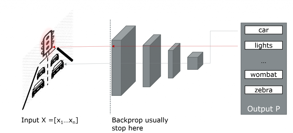
So, saliency maps give us a relevant quantification for every input pixel with respect to a certain class prediction P_i. The pixels important for a traffic light prediction should aggregate around a traffic light. Otherwise, there is something very weird going on.

The good thing about saliency maps is: Because they only rely on gradients calculations, all the commonly used AI frameworks are capable of giving us the saliency maps almost for free. We don’t have to modify the network architectures at all, we just have to modify the gradient calculations a little bit.

Saliency maps in code

We will do step-by-step walkthroughs with the DenseNet 201 architecture, pre-trained on ImageNet. But you take any other. We will show how to get the basic saliency maps with the two most common DL frameworks: PyTorch and TensorFlow 2.x. During the 2 tutorials, we use the Wikipedia lion image as a test image:

Saliency map TensorFlow code

Try it yourself: Code in Colab and GitHub. Free feel to test/rate/feedback it!

We first start by instantiating a DenseNet with ImageNet weights. We can load any images on the disk with the small helper functions and prepare them for feeding to the DenseNet.

import tensorflow as tf
import numpy as np
import matplotlib.pyplot as plt

def prep_input(path):
    image = tf.image.decode_png(tf.io.read_file(path))
    image = tf.expand_dims(image, axis=0)
    image = tf.cast(image, tf.float32)
    image = tf.image.resize(image, [224,224])
    #image = tf.keras.applications.vgg16.preprocess_input(image)
    return image

def norm_flat_image(img):
    grads_norm = img[:,:,0]+ img[:,:,1]+ img[:,:,2]
    grads_norm = (grads_norm - tf.reduce_min(grads_norm))/ (tf.reduce_max(grads_norm)- tf.reduce_min(grads_norm))
    return grads_norm

def plot_maps(img1, img2,vmin=0.3,vmax=0.7, mix_val=2):
    f = plt.figure(figsize=(15,45))
    plt.subplot(1,3,1)
    plt.imshow(img1,vmin=vmin, vmax=vmax, cmap="gray")
    plt.axis("off")
    plt.subplot(1,3,2)
    plt.imshow(img2, cmap = "gray")
    plt.axis("off")
    plt.subplot(1,3,3)
    plt.imshow(img1*mix_val+img2/mix_val, cmap = "gray" )
    plt.axis("off")

When we run inference with the lion test image, we get a prediction vector back.

input_img = prep_input(img_path)
input_img = tf.keras.applications.densenet.preprocess_input(input_img)
plt.imshow(norm_flat_image(input_img[0]), cmap = "gray")
result = test_model(input_img)
max_idx = tf.argmax(result,axis = 1)
tf.keras.applications.imagenet_utils.decode_predictions(result.numpy())

[[('n02129165', 'lion', 0.9963644),
  ('n02106030', 'collie', 0.0027501779),
  ('n02105855', 'Shetland_sheepdog', 0.00042291745),
  ('n02130308', 'cheetah', 0.00014136593),
  ('n02412080', 'ram', 5.228226e-05)]]

And voilà, it peaks at the lion entry with 99.6% confidence. That’s good! But the question is, what made the network so sure about its lion prediction. The partial derivative of the saliency map in this case is:

SaliciencyMap = \frac{dP_{lion}}{dX}

All we have to do is to remember the index entry to identify the lion prediction P_lion in the result vector P. TensorFlow offers the GradientTape function to manage backpropagation-related functions. Within the tape-statement, we define the to-be-watched variables. In particular, we define the variables we are interested in:

• Input input_img <=> X
• Most confident label confidence max_score <=> P_lion

with tf.GradientTape() as tape:
    tape.watch(input_img)
    result = test_model(input_img)
    max_score = result[0,max_idx[0]]
grads = tape.gradient(max_score, input_img)
plot_maps(norm_flat_image(grads[0]), norm_flat_image(input_img[0]))

Calling tape.gradient gives us the desired values. That’s it! Congratulations, you just computed a saliency map. Let’s dive into it:

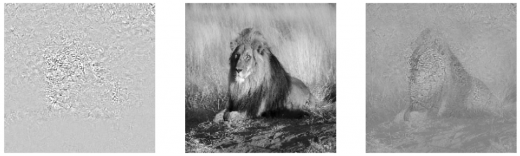
In the saliency map, we can recognize the general shape of the lion. In particular, the highest gradients are around the lion’s face. We have applied a pretty simple normalization and windowing function. Tools like napari are useful (heads-up: napari doesn’t work in Colab) to play around with the contrast and brightness settings.

import napari
viewer = napari.view_image(norm_flat_image(grads[0]))
viewer.add_image(input_img)

Anyway, back to the saliency map: It is conclusive. The classifier indeed looks at the lion… But the map is still very noisy and the shape of the lion is hard to recognize! Perhaps the saliency maps are better with PyTorch?

Saliency map PyTorch code

Try it yourself: The code for the PyTorch example can be found here: Colab or GitHub.

Similar to TensorFlow, we need to do some pre- and postprocessing to feed data to the network:

import torch
import torchvision
from PIL import Image
import numpy as np
import matplotlib.pyplot as plt

def prep_input(path):
    image =Image.open(path)

    preprocess = torchvision.transforms.Compose([
    torchvision.transforms.Resize(256),
    torchvision.transforms.CenterCrop(224),
    torchvision.transforms.ToTensor(),
    torchvision.transforms.Normalize(mean=[0.485, 0.456, 0.406], std=[0.229, 0.224, 0.225]),])

    image = preprocess(image)
    image.unsqueeze_(0)

    return image

def decode_output(output):
    # taken and modified from https://pytorch.org/hub/pytorch_vision_alexnet/
    import urllib.request
    url = "https://raw.githubusercontent.com/pytorch/hub/master/imagenet_classes.txt"
    urllib.request.urlretrieve(url, "imagenet_classes.txt")
    # Read the categories
    probabilities = torch.nn.functional.softmax(output[0], dim=0)

    with open("imagenet_classes.txt", "r") as f:
        categories = [s.strip() for s in f.readlines()]
    # Show top categories per image
    top5_prob, top5_catid = torch.topk(probabilities, 5)
    for i in range(top5_prob.size(0)):
        print(categories[top5_catid[i]], top5_prob[i].item())
    return top5_catid[0]

def prep_output(img_tensor):
    invTrans = torchvision.transforms.Compose([ torchvision.transforms.Normalize(mean = [ 0., 0., 0. ],
                                                    std = [ 1/0.229, 1/0.224, 1/0.225 ]),
                            torchvision.transforms.Normalize(mean = [ -0.485, -0.456, -0.406 ],
                                                    std = [ 1., 1., 1. ]),
                            ])
    out = invTrans(img_tensor)[0]
    out = out.detach().numpy().transpose(1, 2, 0)

    return out



def plot_maps(img1, img2,vmin=0.3,vmax=0.7, mix_val=2):
    f = plt.figure(figsize=(15,45))
    plt.subplot(1,3,1)
    plt.imshow(img1,vmin=vmin, vmax=vmax, cmap="gray")
    plt.axis("off")
    plt.subplot(1,3,2)
    plt.imshow(img2, cmap = "gray")
    plt.axis("off")
    plt.subplot(1,3,3)
    plt.imshow(img1*mix_val+img2/mix_val, cmap = "gray" )
    plt.axis("off")

def norm_flat_image(img):
    grads_norm = prep_output(img)
    grads_norm = grads_norm[:,:,0]+ grads_norm[:,:,1]+ grads_norm[:,:,2]
    grads_norm = (grads_norm - np.min(grads_norm))/ (np.max(grads_norm)- np.min(grads_norm))
    return grads_norm

Now, we can load the DenseNet. Again, you can change the model for any other classifier.

test_model = torchvision.models.densenet201(True)
test_model.eval()
input_img = prep_input("lion.jpg")

In PyTorch, there is a similar auto differentiation mechanism like in TensorFlow for calculating the gradients. First, we have to tell PyTorch, which variables we want to keep in the gradients. Afterward, we can perform a backpropagation and gather the gradients:

# enforce gradient calculation for the input_img
input_img.requires_grad = True
# forward/inference
out = test_model(input_img)
best_id = decode_output(out)
# backprop
out[0, best_id].backward()
grads = input_img.grad
plot_maps(norm_flat_image(grads),norm_flat_image(input_img) )

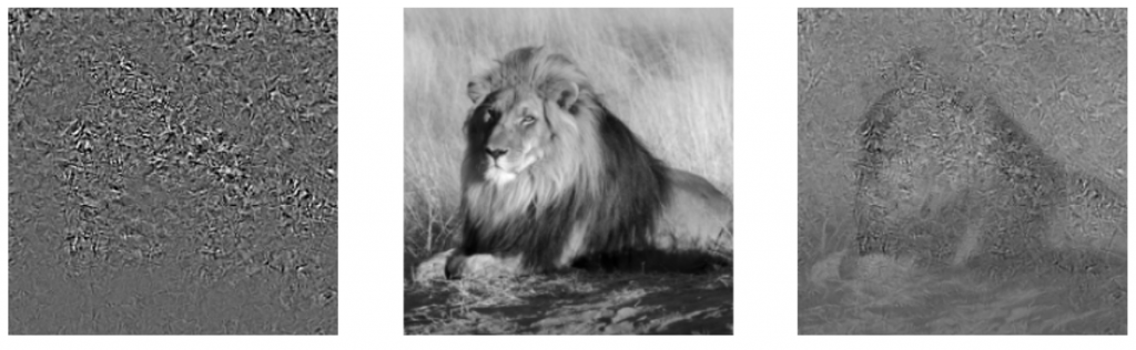
Ok, this is kind of excepted: The saliency map example in PyTorch yields similar results like TensorFlow. We can see the rough shape of the input lion. Still, it is noisy and hard to see. Ok, we have to fix that. In our next blog post, we show a better method: guided backpropagation!

Conclusion/ TL;DR

• We show a hands-on of how to implement (basic) saliency maps in TensorFlow and PyTorch
• Saliency maps are based on gradients and backpropagation
• Basic saliency maps give you a rough understanding of what an AI is looking at
• They shows rough shapes of important features, but are still very noisy
• Stay tuned, we will fix the noisy saliency maps!

References and further readings

• Simonyan et al.: Deep Inside Convolutional Networks: Visualising Image Classification Models and Saliency Maps (2014)
• Springenberg, Dosovitskiy et al.: Striving for Simplicity: The All Convolutional Net (2015)
• How-to: Guided Backpropagation with PyTorch and TensorFlow